Using xgbfi for revealing feature interactions

Tree based methods excel in using feature or variable interactions. As a tree is built, it picks up on the interaction of features. For example, buying ice cream may not be affected by having extra money unless the weather is hot. It is the interaction of both of these features that can affect whether ice cream will be consumed.

The traditional manner for examining interactions is relying on measures of variable importance. However, these measures don’t provide insights into second or third order interactions. Identifying these interactions are important in building better models, especially when finding features to use within linear models.

In this post, I show how to find higher order interactions using XGBoost Feature Interactions & Importance. This tool has been available for a while, but outside of kagglers, it has received relatively little attention.

As a starting point, I used the Ice Cream dataset to illustrate using xgbfi. This walkthrough is in R, but python instructions are also available at the repo. I am going to break the code into three sections, the initial build of the model, exporting the files necessary for xgbfi, and running xgbi.

Building the model

Lets start by loading the data:

library(xgboost)
library(Ecdat)
data(Icecream)
train.data <- data.matrix(Icecream[,-1])

The next step is running xgboost:

bst <- xgboost(data = train.data, label = Icecream$cons, max.depth = 3, eta = 1, nthread = 2, nround = 2, objective = "reg:linear")

To better understand how the model is working, lets go ahead and look at the trees:

xgb.plot.tree(feature_names = names((Icecream[,-1])), model = bst)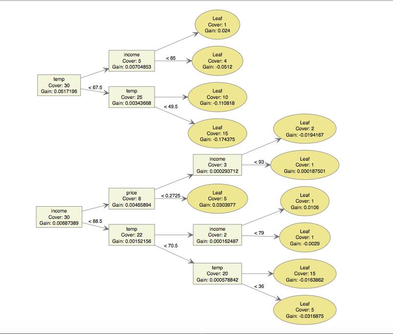

The results here line up with our intution. Hot days seems to be the biggest variable by just eyeing the plot. This lines up with the results of a variable importance calculation:

> xgb.importance(colnames(train.data, do.NULL = TRUE, prefix = "col"), model = bst)
   Feature       Gain      Cover Frequency
1:    temp 0.75047187 0.66896552 0.4444444
2:  income 0.18846270 0.27586207 0.4444444
3:   price 0.06106542 0.05517241 0.1111111

All of this should be very familiar to anyone who has used decision trees for modeling. But what are the second order interactions? Third order interactions? Can you rank them?

Exporting the tree

The next step involves saving the tree and moving it outside of R so xgbfi can parse the tree. The code below will help to create two files that are needed:xgb.dump and fmap.text.

featureList <- names(Icecream[,-1])
featureVector <- c() 
for (i in 1:length(featureList)) { 
  featureVector[i] <- paste(i-1, featureList[i], "q", sep="\t") 
}
write.table(featureVector, "fmap.txt", row.names=FALSE, quote = FALSE, col.names = FALSE)
xgb.dump(model = bst, fname = 'xgb.dump', fmap = "fmap.txt", with.stats = TRUE)

Running xgbfi

The first step is to clone the xgbfi repository onto your computer. Then copy the files xgb.dump and fmap.text to the bin directory.

Go to your terminal or command line and run: XgbFeatureInteractions.exe application. On a mac, download mono and then run the command: mono XgbFeatureInteractions.exe. There is also a XgbFeatureInteractions.exe.config file that contains configuration settings in the bin directory.

After the application runs, it will write out an excel spreadsheet titled: XgbFeatureInteractions.xlsx. This spreadsheet has the good stuff! Open up the spreadsheet and you should see:

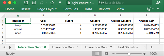
This tab of the spreadsheet shows the first order interactions. These results are similar to what variable importance showed. The good stuff is when you click on the tab for Interaction Depth 1 or Interaction Depth 2.

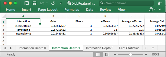
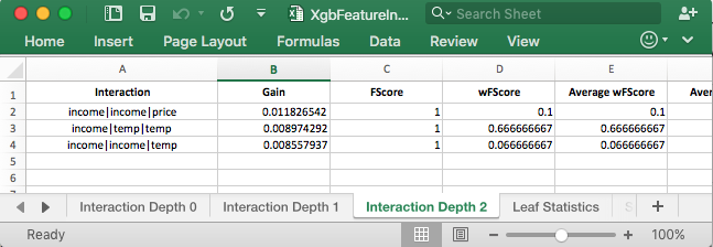
It is now possible to rank the higher order interactions. With the simple dataset, you can see that the results out of xgbfi match what is happening in the tree. The real value of this tool is for much larger datasets, where its difficult to examine the trees for the interactions.