Optimization Strategies

As a data scientist, you spend a lot of your time helping to make better decisions. You build predictive models to provide improved insights. You might be predicting whether an image is a cat or dog, store sales for the next month, or the likelihood if a part will fail. In this post, I won’t help you with making better predictions, but instead how to make the best decision.

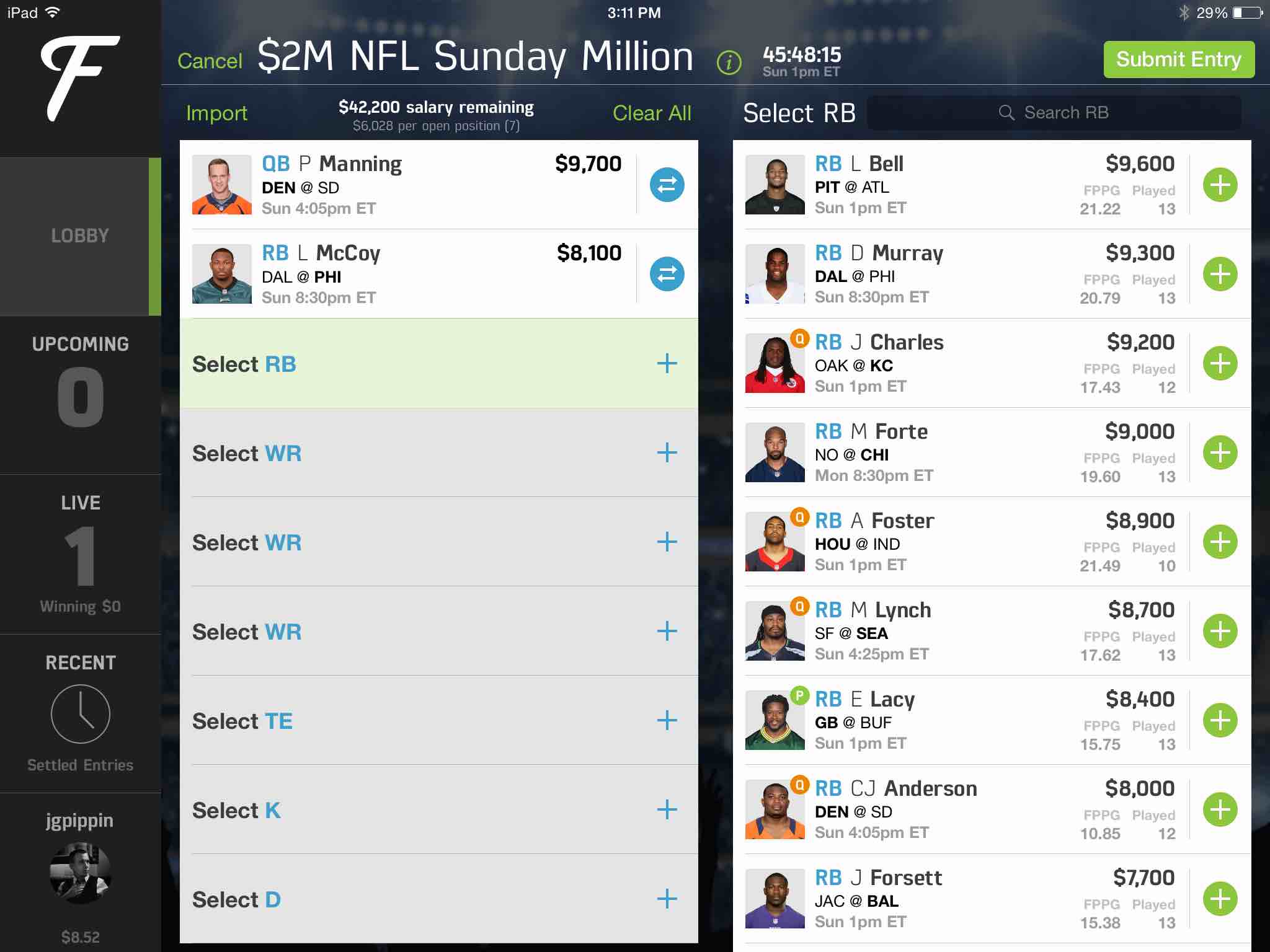
The post strives to give you some background on optimization. It starts with a simply toy example show you the math behind an optimization calculation. After that, this post tackles a more sophisticated optimization problem, trying to pick the best team for fantasy football. The FanDuel image below is a very common sort of game that is widely played (ask your inlaws). The optimization strategies in this post were shown to consistently win! Along the way, I will show a few code snippets and provide links to working code in R, Python, and Julia. And if you do win money, feel free to share it :)

Simple Optimization Example

A simple example, which I found online, starts with a carpenter making bookcases in two sizes, large and small. It takes 6 hours to make a large bookcase and 2 hours to make a small one. The profit on a large bookcase is $50, and the profit on a small bookcase is $20. The carpenter can spend only 24 hours per week making bookcases and must make at least 2 of each size per week. Your job as a data scientist is to help your carpenter maximize her revenue.

Your initial inclination could be that since the large bookcase is the most profitable, why not focus on them. In that case, you would profit (2*$20) + (3*$50) which is $190. That is a pretty good baseline, but not the best possible answer. It is time to get the algebra out and create equations that define the problem. First, we start with the constraints:

x>=2    ## large bookcases

y>=2    ## small bookcases

6x + 2y <= 24  (labor constraint)

Our objective function which we are trying to maximize is:

P = 50x + 20y

If we do the algebra by hand, we can convert out constraints to y <= 12 - 3x. Then we graph all the constraints and find the feasible area for the portion of making small and large bookcases:

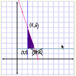
The next step is figuring out the optimal point. Using the corner-point principle of linear programming, the maximum and minimum values of the objective function each occur at one of the vertices of the feasible region. Looking here, the maximum values (2,6) is when we make 2 large bookcases and 6 small bookcases, which results in an income of $220.

This is a very simple toy problem, typically there are many more constraints and the objective functions can get complicated. There are lots of classic problems in optimization such as routing algorithms to find the best path, scheduling algorithms to optimize staffing, or trying to find the best way to allocate a group of people to set of tasks. As a data scientist, you need to dissect what you are trying to maximize and identify the constraints in the form of equations. Once you can do this, we can hand this over to a computer to solve. So lets next walk through a bit more complicated example.

Fantasy Football

Over the last few years, fantasy sports have increasingly grown in popularity. One game is to pick a set of football players to make the best possible team. Each football player has a price and there is a salary cap limit. The challenge is to optimize your team to produce the highest total points while staying within a salary cap limit. This type of optimization problem is known as the knapsack problem or an assignment problem.

Simple Linear Optimization

So for this problem, let’s start by loading a dataset and taking a look at the raw data. You need to know both the salary as well as the expected points. Most football fans spend a lot of time trying to predict how many points a player will score. If you want to build a model for predicting the expected performance of a player, take a look at Ben’s blog post.

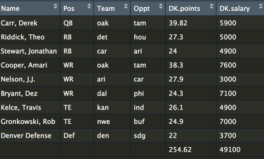
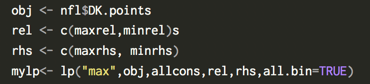
The goal here is to build the best possible team for a salary cap, let’s say $50,000. A team consists of a quarterback, running backs, wide receivers, tight ends, and a defense. We can use the lpSolve package in R to set up the problem. Here is a code snippet for setting up the constraints.

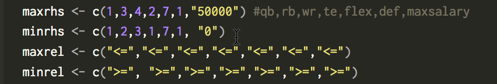
If you parse through this, you can see we have set a minimum and maximum for QB of 1 player. However, for the RB, we have allowed a maximum of 3 and a minimum of 2. This is not unusual in fantasy football, be because there is a role called a flex player, which anyone can choose and they can either be a RB, WR, or TE. Now let’s look at the code for the objective:

The code shows that we have set up the problem to maximize the objective of the most points and include our constraints. Once the code is run, it outputs an optimal team! I forked an existing repo and have made the R code and dataset are available here. A more sophisticated python optimization repo is also available.

Advanced steps

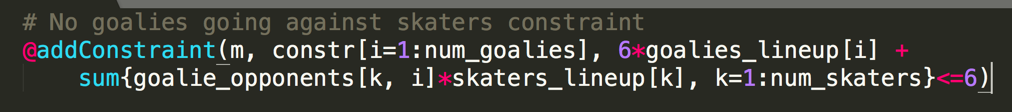
So far, we have built a very simple optimization to solve the problem. There are several other strategies to further improve the optimizer. First, the variance of our teams can be increased by using a strategy called stacking, where you make sure your QB and WR are on the same team. A simple optimization is a constraint for selecting a QB and WR from the same team. Another strategy is using an overlap constraint for selecting multiple lineups. An overlap constraint ensures a diversity of players and not the same set of players for each optimized team. This strategy is particularly effective when submitting multiple lineups. You can read more about these strategies here and run the code in Julia here. An code snippet of the stacking constraint (this is for a hockey optimization):

.

Last year, at Sloan sports conference, Haugh and Sighal , presented a paper with additional optimization constraints. They include what an opponents team is likely to look like. After all, there are some players that are much more popular. Using this knowledge, you can predict the likely teams that will oppose your team. The approach here used Dirichlet regressions for modeling players. The result was a much-improved optimizer that was capable of consistently winning!

I hope this post has shown you how optimization strategies can help you find the best possible solution.

​