Your boss hands you a pile of a 100,000 unlabeled images and asks you to categorize whether they are sandals, pants, boots, etc.
So now you have a massive set of unlabeled data and you need labels. What should you do?
This problem is commonplace. Lots of companies are swimming with data, whether its transactional, IoT sensors, security logs, images, voice, or more, and its all unlabeled. With so little labeled data, it is a tedious and slow process for data scientists to build machine learning models in most all enterprises.
Take Google’s street view data. Gebru had to figure out how to label cars in 50 million images with very little labeled data. Over at Facebook, they used algorithms to label half a million videos, a task that would have otherwise taken 16 years.
This post shows you how to label hundreds of thousands of images in an afternoon. You can use the same approach whether you are labeling images or labeling traditional tabular data (e.g, identifying cyber security atacks or potential part failures.)
The Manual Method
For most data scientists when asked to do something, the first step is to calculate who else should do this.

But 100,000 images could cost you at least $30,000 on Mechanical Turk or some other competitor. Your boss expects this done cheaply, since after all, they hired you because you use free software. Now, she doesn’t budget for anything other than your salary (if you don’t believe me, ask to go to pydata).
You take a deep breath and figure you can probably label 200 images in an hour. So that means in three weeks of non stop work, you can get this done!! Yikes!
Just Build a Model
The first idea is to label a handful of the images, train a machine learning algorithm, and then predict the remaining set of labels. For this exercise, I am using the Fashion-MNIST dataset (you could also make your own using quickdraw). There are ten classes of images to identify and here is a sample of what they look like:
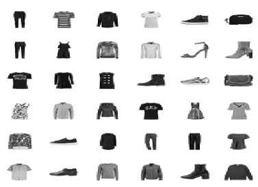
I like this dataset, because each image is 28 by 28 pixels, which means it contains 784 unique features/variables. For a blog post this works great, but its also not like any datasets you see in the real world, which are often either much narrower (traditional tabluar business problem datasets) or much wider (real images are much bigger and include color).
I built models using the most common data science algorithms: logistic regression, support vector machines (SVM), random forest and gradient boosted machines (GBM).
I evaluated the performance based on labeling 100, 200, 500, 1000, and 2000 images.
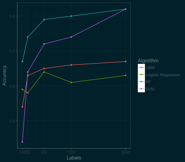
At this point in the post, if you are still with me, slow down and mull this graph over. There is a lot of good stuff here. Which algorithm does the best? (If you a data scientist, you shouldn’t fall for that question.) It really depends on the context.
You want something quick and dependable out of the box, you could go for the logistic regression. While the random forest starts way ahead, the SVM is coming on fast. If we had more labeled data the SVM would pass the random forest. And the GBM works great, but can take a bit of work to perform their best. The scores here are using out of the box implementations in R (e1071, randomForest, gbm, nnet).
If our benchmark is 80% accuracy for ten classes of images, we could get there by building a Random Forest model with 1000 images. But 1000 images is still a lot of data to label, 5 hours by my estimate. Lets think about ways we can improve.
Let’s Think About Data
After a little reflection, you remember what you often tell others — that data isn’t random, but has patterns. By taking advantage of these patterns we can get insight in our data.
Lets start with an autoencoder (AE). An autoencoder squeezes and compresses your data, kind of like turning soup into a bouillon cube. Autoencoders are the hipster’s Principle Component Analysis (PCA) , since they support nonlinear transformations.
Effectively this means we are taking our wide data (784 features/variables) reducing it down to 128 features. We then take this new compressed data and train our machine learning algorithm (SVM in this case). The graph below shows the difference in performance between an SVM fed with an autoencoder (AE_SVM) versus the SVM on the raw data.
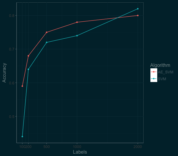
By squeezing the information down to 128 features, we were able to actually improve the performance of the SVM algorithm at the low end. At the 100 labels mark, accuracy went from 44% to 59%. At the 1000 labels mark, the autoencoder was still helping, we see an improvement from 74% to 78%. So we are on to something here. We just need think a bit more about the distribution and patterns in our data that we can take advantage of.
Thinking Deeper About Your Data
We know that our data are images and since 2012, the hammer for images is a convolutional neural network (CNN). There are a couple of ways we could use a CNN, from a pretrained network or as a simple model to pre-process the images. For this post, I am going to use a Convolutional Variational Autoencoder as a path towards the technique by Kingma for semi-supervised learning.
So lets build a Convolutional Variational Autoencoder (CVAE). The leap here is twofold. First, “variational” means the autoenconder compress the information down into a probability distribution. Second is the addition of using a convolutional neural networks as an encoder. This is a bit of deep learning, but the emphasis here is on how we are solving the problem, not the latest shiny toy.
For coding my CVAE, I used the example CVAE from the list of examples over at RStudio’s Keras page. Like the previous autoencoder, we design the latent space to reduce the data to 128 features. We then use this new data to train an SVM model. Below is a plot of the performance of the CVAE as compared to the SVM and RandomForest on the raw data.
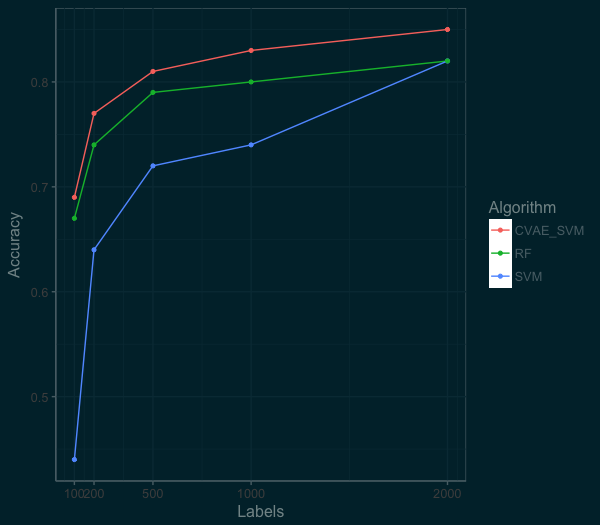
Wow! The new model is much more accurate. We can get well past 80% accuracy with just 500 labels. By using these techniques we get better performance and require less labelled images! At the top end, we can also do much better than the RandomForest or SVM model.
Next Steps
By using some very simple semi-supervised techniques with autoencoders, its possible to quickly and accurately label data. But the takeaway is not to use deep learning auto encoders! Instead, I hope you understand the methodology here of starting very simple and then trying gradually more complex solutions. Don’t fall for the latest shiny toy — pratical data science is not about using the latest approaches found in arxiv.
If this idea of semi-supervised learning inspires you, this post is the logistic regression of semi-supervised learning. If you want to dig further into Semi-Supervised Learning and Domain Adaptation, check out Brian Keng’s great walkthrough of using variational autoencoders (which goes beyond what we have done here) or the work of Curious AI, which has been advancing semi-supervised learning using deep learning and sharing their code. But at the very least, don’t reflexively think all your data has to be hand labeled.